The Excel VLOOKUP function is a powerful tool used to search for a value in the first column of a table and return a value in the same row from another column. This function is especially useful for large datasets where you need to quickly find related information.
Syntax
| Function | Description |
|---|---|
| VLOOKUP(lookup_value, table_array, col_index_num, [range_lookup]) | Searches for a value in the first column of a table array and returns a value in the same row from a specified column. |
Parameters
- lookup_value: The value you want to search for in the first column of the table array.
- table_array: The range of cells that contains the data you want to search.
- col_index_num: The column number in the table array from which to retrieve the value.
- range_lookup (optional): A logical value that specifies whether you want an exact match (FALSE) or an approximate match (TRUE).
Example
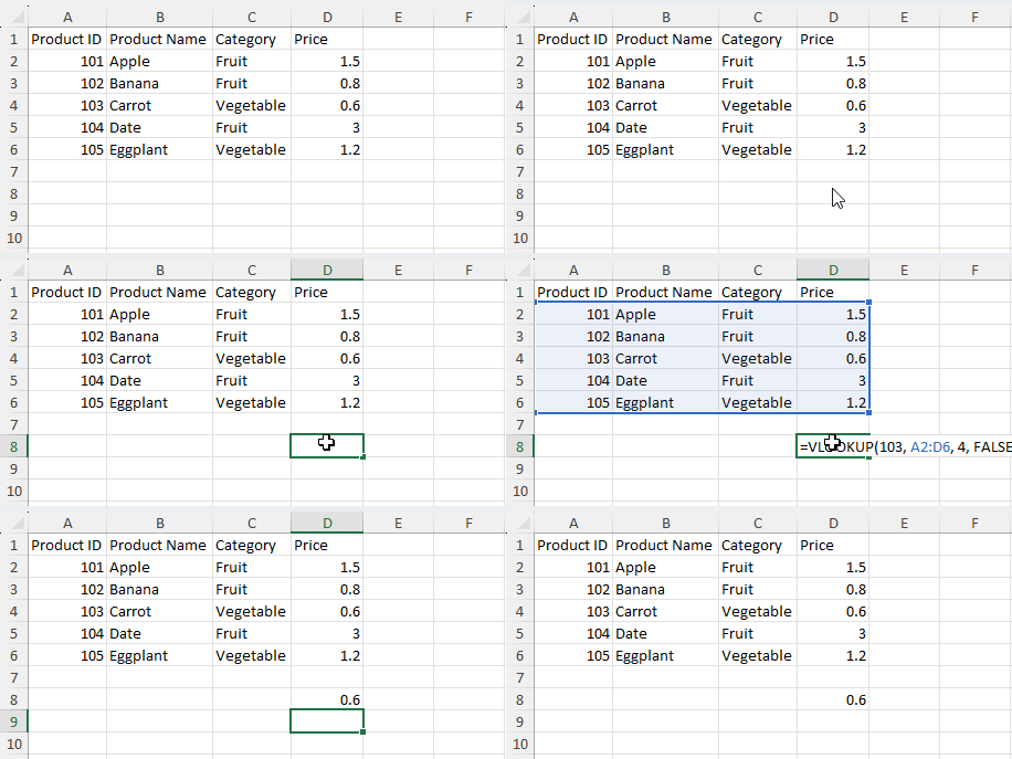
Let's consider an example to demonstrate how the VLOOKUP function works.
Task: We want to find the price of the product with Product ID 103.
=VLOOKUP(103, A2:D6, 4, FALSE)This formula will return 0.60, which is the price of the product with Product ID 103.

Practice
Practice Exercise 1
Task: Find the product name and category of the product with Product ID 104.
Practice Exercise 2
Task: Find the price of the product named "Eggplant".
Solutions
A Solution to Practice Exercise 1
To find the product name and category of the product with Product ID 104:
Formula for Product Name:
=VLOOKUP(104, A2:D6, 2, FALSE)This formula will return "Date".
Formula for Category:
=VLOOKUP(104, A2:D6, 3, FALSE)This formula will return "Fruit".
A Solution to Practice Exercise 2
To find the price of the product named "Eggplant":
=VLOOKUP("Eggplant", B2:D6, 3, FALSE)This formula will return 1.20, which is the price of the product named "Eggplant".