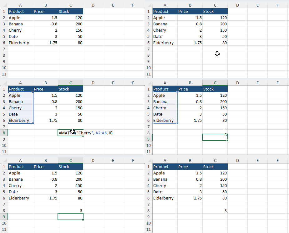
The Excel MATCH function is a versatile tool used to find the position of a specific value in a range or array. It is particularly useful for situations where you need to locate an item's position in a list, rather than the item itself. MATCH can be used with other functions, such as INDEX, to perform complex lookups.
Syntax
| Function | Description |
|---|---|
| MATCH(lookup_value, lookup_array, [match_type]) | Returns the relative position of an item in an array that matches a specified value. |
Parameters
- lookup_value: The value you want to search for.
- lookup_array: The range of cells or array to search within.
- match_type (optional): The number -1, 0, or 1. The match type specifies how Excel matches the lookup_value with values in the lookup_array.
Match Types
- 1: Finds the largest value that is less than or equal to the lookup_value. The lookup_array must be sorted in ascending order.
- 0: Finds the first value that is exactly equal to the lookup_value. The lookup_array does not need to be sorted.
- -1: Finds the smallest value that is greater than or equal to the lookup_value. The lookup_array must be sorted in descending order.
Example
Task: We want to find the position of "Cherry" in the Product column.
=MATCH("Cherry", A2:A6, 0)This formula will return 3, indicating that "Cherry" is the third item in the range A2.

Exercises
Practice Exercise 1
Task: Find the position of the product with the price of 1.75 in the Price column.
Practice Exercise 2
Task: Find the position of the product with the highest stock in the Stock column.
Solutions
A Solution to Practice Exercise 1
To find the position of the product with the price of 1.75:
Formula:
=MATCH(1.75, B2:B6, 0)This formula will return 5, indicating that the price of 1.75 is the fifth item in the range B2.
A Solution to Practice Exercise 2
To find the position of the product with the highest stock:
Formula:
=MATCH(MAX(C2:C6), C2:C6, 0)This formula will return 2, indicating that the highest stock value is the second item in the range C2.